Tutorial: analyzing presidential elections

Before you start:

Make sure you’ve installed RethinkDB—it should only take a minute!

Given the timeliness of the 2012 US Presidential Election and the inherent intricacies of the electoral process, we internally used an interesting dataset on poll results to test RethinkDB’s query language support in the JavaScript, Python, and Ruby client libraries.

We’ll use this dataset to walk through RethinkDB’s JavaScript query language using the Data Explorer.

If you want to do follow the tutorial with the node driver:

If you have not done it yet, you may want to read the 10 minute guide.

Import the data

Download the datasets:

wget https://raw.github.com/rethinkdb/rethinkdb/next/demos/election/input_polls.json
wget https://raw.github.com/rethinkdb/rethinkdb/next/demos/election/county_stats.json

Import them in RethinkDB:

rethinkdb import -c localhost:28015 --table test.input_polls --pkey uuid -f input_polls.json --format json
rethinkdb import -c localhost:28015 --table test.county_stats --pkey uuid -f county_stats.json --format json

What does this data set contain?

You have imported two tables:

input_polls contains multiple poll results at state-level
county_stats contains various population stats at county-level

You can take a look at the documents in each set with these queries:

r.table('input_polls').limit(1)

The result returned should be something similar to:

[{
    "uuid":"001b1830-b786-402e-a10b-1c3ea225971d",
    "id":"New Hampshire",
    "Pollster":"Marist Coll.-2",
    "Len":2,
    "GOP":45,
    "EV":4,
    "Dem":45,
    "Day":175.5,
    "Date":"Jun 25"
}]

For the table county_stats:

r.table('county_stats').limit(1)

You will get back something with this schema:

[{
    "uuid":"0052158f-6f15-4c27-851d-447b76c587ba",
    "state":"17",
    "ctyname":"Champaign County",
    "county":"019",
    "Stname":"Illinois",
    "SUMLEV":"050",
    "Rdeath2011":5.8652045006,
    "Rbirth2011":11.775067919000001,
    "RNETMIG2011":-4.406346528,
    "RNATURALINC2011":5.9098634181000005,
    "RINTERNATIONALMIG2011":3.8009700909,
    "RESIDUAL2011":12,
    "RESIDUAL2010":1,
    "REGION":2,
    "RDOMESTICMIG2011":-8.207316619,
    "POPESTIMATE2011":201685,
    "POPESTIMATE2010":201370,
    "NPOPCHG_2011":315,
    "NPOPCHG_2010":289,
    "NETMIG2011":-888,
    "NETMIG2010":-59,
    "NATURALINC2011":1191,
    "NATURALINC2010":347,
    "INTERNATIONALMIG2011":766,
    "INTERNATIONALMIG2010":207,
    "GQESTIMATESBASE2010":16129,
    "GQESTIMATES2011":16129,
    "GQESTIMATES2010":16129,
    "ESTIMATESBASE2010":201081,
    "Deaths2011":1182,
    "Deaths2010":270,
    "DOMESTICMIG2011":-1654,
    "DOMESTICMIG2010":-266,
    "DIVISION":3,
    "CENSUS2010POP":201081,
    "Births2011":2373,
    "Births2010":617
}]

Data cleanup: chaining, group-map-reduce, simple map

We’ll first clean up the data in input_polls, as we want to calculate the average results of various polls at the state level. We’ll also get rid of unnecessary/empty attributes. Finally we’ll store the result in a new table:

First let’s create a new table that will contain the clean data.

r.db("test").tableCreate("polls")

Then let’s rework the data and save it in polls. We are going to group polls per state and compute the average score for each party.

r.table("polls").insert(
    r.table("input_polls")
     .group("id")         // We group the table by `id`, which is the state name.
     .pluck('Dem', 'GOP') // We pluck out the poll results we care about.
     .merge({polls: 1})   // And finally, we add an extra field `polls: 1` to each row.
     .reduce(function(left, right){
        // We reduce over the polls, adding up the results and keeping
        // track of the total number of polls.
        return {
            Dem: left("Dem").add(right("Dem")),
            GOP: left("GOP").add(right("GOP")),
            polls: left("polls").add(right("polls"))
        };
     }).ungroup().map(function(state){
         // We ungroup and divide the fields `Dem` and `GOP` for each state
         // by the number of polls to get the average result per state.
         return {
             Dem: state("reduction")("Dem").div(state("reduction")("polls")),
             GOP: state("reduction")("GOP").div(state("reduction")("polls")),
             polls: state("reduction")("polls"),
             id: state("group")
         };
     })
)

If everything went well, you should see that we inserted 51 documents (one per state plus one for Washington DC).

{
    "unchanged":0,
    "skipped":0,
    "replaced":0,
    "inserted":51,
    "errors":0,
    "deleted":0
}

If you take a look at the Arizona state

r.table('polls').get("Arizona")

You should get back this document:

{
	"Dem": 42.294117647058826,
	"GOP": 48.294117647058826,
	"polls": 17,
	"id": "Arizona"
}

Data analysis: projections, JOINs, orderby, group-map-reduce

Based on this data let’s try to see if we can figure out how many voters a party would need to turn to win the states. For the sake of this post, we’ll go with the Democrats.

Let’s start with what estimates polls project at the county level by JOINing the polls and county_stats tables:

r.table('county_stats').eqJoin('Stname', r.table('polls')) // equi join of the two tables
	.zip() // flatten the results
	.pluck('Stname', 'state', 'county', 'ctyname', 'CENSUS2010POP', 'POPESTIMATE2011', 'Dem', 'GOP') // projection

Building on this query, next we can find the counties where the Democrats are in minority:

r.table('county_stats').eqJoin('Stname', r.table('polls'))
	.zip()
	.pluck('Stname', 'state', 'county', 'ctyname', 'CENSUS2010POP', 'POPESTIMATE2011', 'Dem', 'GOP')
	.filter(function(doc) { return doc('Dem').lt(doc('GOP')) })

Or even better where Democrats are within 15% of the Republicans:

r.table('county_stats').eqJoin('Stname', r.table('polls'))
	.zip()
	.pluck('Stname', 'state', 'county', 'ctyname', 'CENSUS2010POP', 'POPESTIMATE2011', 'Dem', 'GOP')
	.filter(function(doc) { return doc('Dem').lt(doc('GOP')).and(doc('GOP').sub(doc('Dem')).lt(15)) })

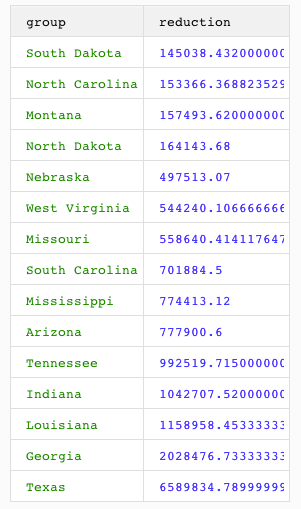
The last step in answering the initial question of how many voters should the Democrats win to turn the results is just a group/map/sum away:

r.table('county_stats').eqJoin('Stname', r.table('polls')).zip()
    .pluck('Stname', 'state', 'county', 'ctyname', 'CENSUS2010POP', 'POPESTIMATE2011', 'Dem', 'GOP')
    .filter(function(doc) { return doc('Dem').lt(doc('GOP')).and(doc('GOP').sub(doc('Dem')).lt(15)) })
    .group('Stname')
    .map(function(doc){return doc('POPESTIMATE2011').mul(doc("GOP").sub(doc("Dem"))).div(100);})
    .sum()

And the outcome of our quick presidential election data analysis that addresses the question how many voters the Democrat party would need to turn to win the states (this assumes 100% turnout of the entire population of a state):

Data analysis with RethinkDB

If you followed along, the queries above should have given you a taste of ReQL: chaining, projections, order by, JOINs, group. Of course this tutorial isn’t statistically significant. If you interested in statistically significant results, checkout the election statistics superhero Nate Silver.